01 — OVERVIEW

Wolfram Mathematica · Amp · Wolfram Quantum Framework · Qiskit

Grand Unification of
Quantum Algorithms

A research paper turned into verified, runnable quantum circuits — an end‑to‑end pipeline that derives Quantum Signal Processing symbolically, checks every identity to machine precision, and exports portable OpenQASM.

QSP → Chebyshev → Hamiltonian simulation

Wolfram Quantum Framework · SecondQuantization

Wolfram ↔ Qiskit agreement 6×10⁻¹⁶

Powered by

·

· OpenQASM

Prepared by

ESL — Engineering Software Lab

Software Engineering Consultants

eswlab.com/contact-us →

Author

Daniel Liezrowice

LinkedIn →

← Swipe / arrow keys to navigate →

02 — THE SUBJECT

One primitive, most known quantum algorithms

Martyn, Rossi, Tan & Chuang, Grand Unification of Quantum Algorithms (PRX Quantum 2, 040203, 2021), building on Low & Chuang (PRL 118, 010501, 2017).

The core insight

Nearly every flagship quantum algorithm is a polynomial transformation of a block‑encoded operator, selected by a sequence of phase angles. That single object is Quantum Signal Processing (QSP) and its lift to matrices, QSVT.

Amplitude amplification / Grover search
Hamiltonian simulation e^−iHt
Quantum linear systems A⁻¹
Phase / eigenvalue estimation
General matrix functions f(A)

Why it matters commercially

Unification moves the hard problem from physics to engineering:

One compiler target serves many algorithms — R&D is amortized.
The bottleneck becomes “find the phase angles” — a numerical, productizable task.
QSVT gives near‑optimal resource scaling — it defines what a machine can actually reach.

The practical needs: derive → verify → generate phases → estimate cost → run anywhere.

03 — THE SOLUTION

The workflow we built

A reproducible pipeline: the paper's mathematics is executed in Wolfram, cross‑checked in Qiskit at machine precision, and handed off through vendor‑neutral OpenQASM.

📄 Paper

QSP / QSVT theory

→

∑ Mathematica

symbolic derivation (.wl/.wls)

→

✓ Verify

identities to ~10⁻¹⁶

→

∠ Phase angles

FindQSPPhases

⟨ OpenQASM ⟩

portable QASM 2 & 3

→

⚛ Qiskit + Aer

circuits · sim · resources

→

◎ Classiq

synthesis hand‑off (next)

→

🖥 Hardware

IBM / IonQ / …

35 / 35proof‑audit checks passed

6.1×10⁻¹⁶Wolfram ↔ Qiskit unitary agreement

0.99999994e⁻ⁱᴴᵗ reconstruction overlap

Toolchain

·

· OpenQASM

04 — THE TOOLCHAIN

Optimal Mathematica, driven by Amp

Wolfram Quantum Framework

The paclet from resources.wolframcloud.com provides the quantum objects. Its SecondQuantization functionality — not a separate paclet — supplies the creation/annihilation operators used to build the Hamiltonian.

a = AnnihilationOperator[n] n̂ = a^† a (* number operator *) H = ω n̂ + g (a + a^†) , ‖H‖ ≤ 1

Headless .wl / .wls scripts

The whole pipeline runs from the command line — no notebook GUI needed — so it is reproducible, scriptable and git‑friendly. Amp's Mathematica skill orchestrates it:

# Amp-driven, three headless stages wolframscript -file build_project.wls # derive+verify+phases python qiskit_pipeline.py # circuits+QASM+sim wolframscript -file proof_audit.wls # 35 checks

An evaluated companion notebook, QSPUnification.nb, is generated for interactive exploration.

Wolfram Language 14.3

QuantumFramework 1.6.5

qiskit 2.5 · aer

resources.wolframcloud.com

05 — THE MATHEMATICS

Quantum Signal Processing in one screen

A single qubit, interleaving a fixed signal rotation with tunable phase rotations, realises a polynomial in the signal a = cos θ.

Signal & phase operators (Wx convention)

W(a) = e^{i·arccos(a)·X} = [ a i√(1−a²) ] [ i√(1−a²) a ] S(φ) = e^i·φ·Z

The QSP sequence & its response

U_Φ(a) = S(φ₀) ∏_k=1..d W(a) S(φ_k) P(a) = ⟨0| U_Φ(a) |0⟩

d signal calls · d+1 phases. Choosing the phases shapes Re P(a) into any target polynomial of degree ≤ d and matching parity.

06 — DERIVATION

QSP ⇒ Chebyshev polynomials

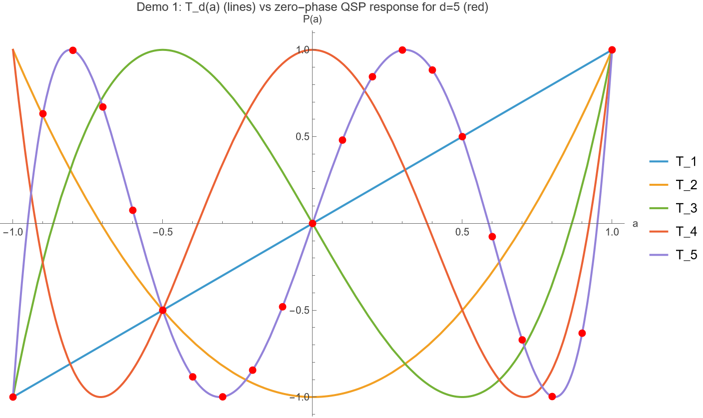
Chebyshev polynomials T_d vs zero-phase QSP response

Wolfram output — T₁…T₅ (lines) vs the zero‑phase QSP response for d=5 (red dots). The dots sit exactly on T₅.

Set every phase to zero and QSP collapses to the Chebyshev polynomials — derived symbolically, not fitted:

φ = 0 ⟹ P(a) = T_d(a), Q(a) = U_d−1(a)

and they obey the Pell / Chebyshev identity exactly:

T_d(a)² + (1 − a²) · U_d−1(a)² = 1

Proven symbolically for d = 1…8
Parity: T_d(−a) = (−1)^d T_d(a)
Numeric match: max error 7.8×10⁻¹⁶

07 — VERIFICATION

Every identity, checked numerically

Nothing is asserted without a test. Symbolic truth is confirmed numerically, then re‑confirmed against an independent tool.

Check	Result
Chebyshev symbolic derivation (d = 1…6)	all pass
Zero‑phase QSP vs T_d, max error	7.77×10⁻¹⁶
QSP unitarity \|P\|²+(1−a²)\|Q\|² = 1	8.88×10⁻¹⁶
Jacobi–Anger cos truncation error	2.15×10⁻¹¹
Jacobi–Anger sin truncation error	1.42×10⁻¹²
Phase generation — cos target	2.79×10⁻⁷
Phase generation — sin target	6.60×10⁻⁸
e^−iHt reconstruction max error	1.34×10⁻⁷
Wolfram ↔ Qiskit unitary agreement (19 checkpoints)	6.12×10⁻¹⁶
Proof audit	35 passed · 0 failed

08 — HAMILTONIAN SIMULATION

From cos & sin to e^−iHt

Time evolution needs QSP to approximate trigonometric functions. The Jacobi–Anger expansion supplies polynomials whose coefficients are Bessel functions:

cos(t·a) = J₀(t) + 2 Σ_k≥1 (−1)^k J_2k(t) T_2k(a)

The Hamiltonian is built from SecondQuantization operators (a driven, truncated‑Fock oscillator), normalised so ‖H‖ ≤ 1, then diagonalised:

eig(H) = { −0.706, −0.311, 0.167, 0.850 }

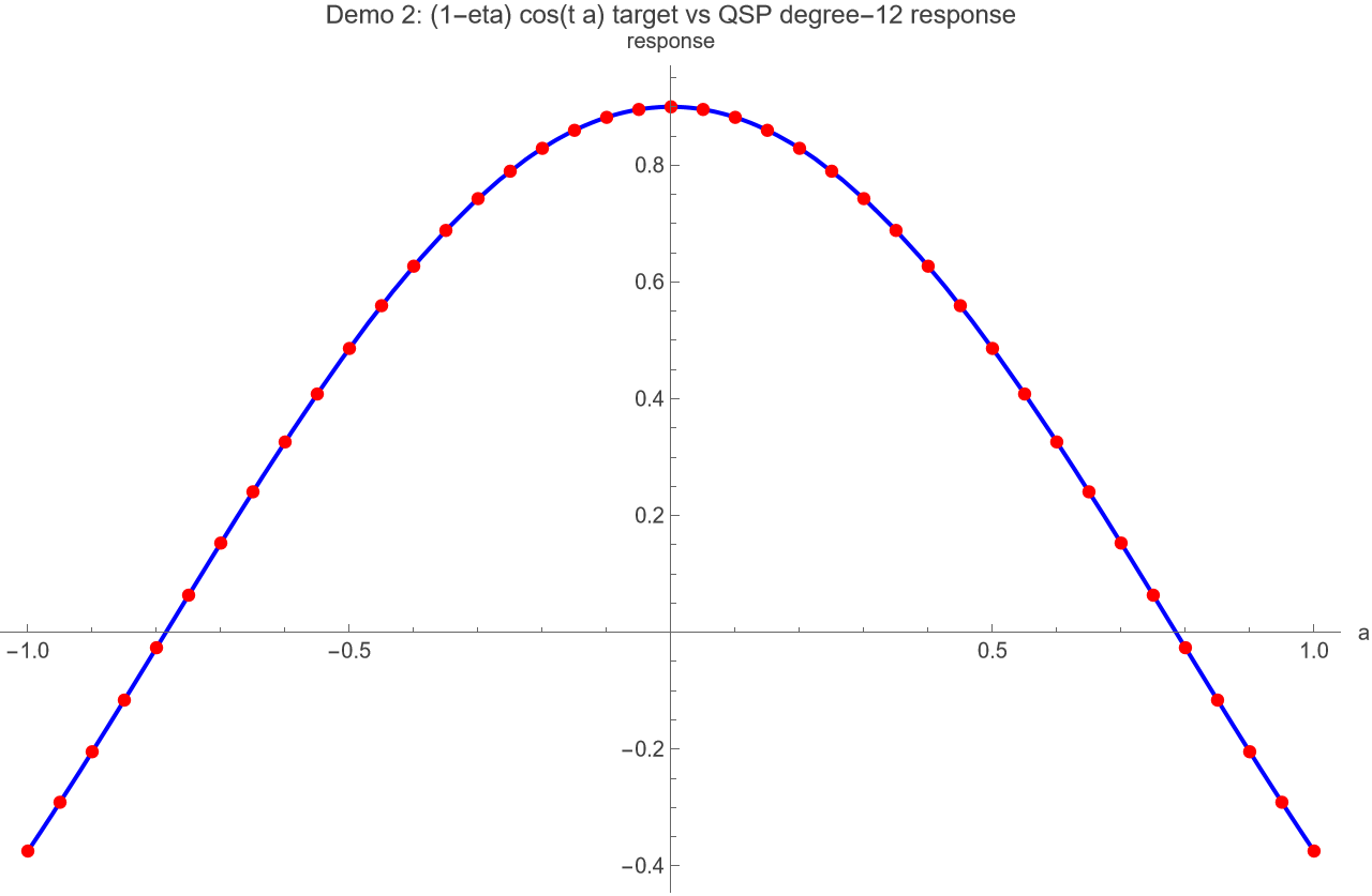
Degree-12 QSP response vs (1-eta) cos(t a) target

Wolfram output — a degree‑12 QSP polynomial (red dots) reproduces the scaled cosine target (1−η)·cos(t·a) across [−1, 1].

09 — RESULT

Eigenvalue transform & reconstruction

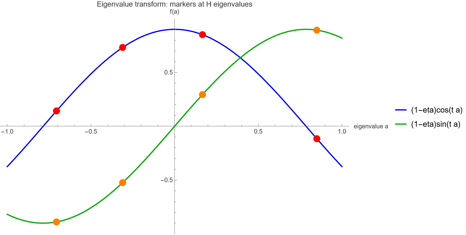
Eigenvalue transform with markers at H eigenvalues

Targets (1−η)cos(t·a) and (1−η)sin(t·a); markers land on the four eigenvalues of H — QSVT transforms each eigenvalue independently.

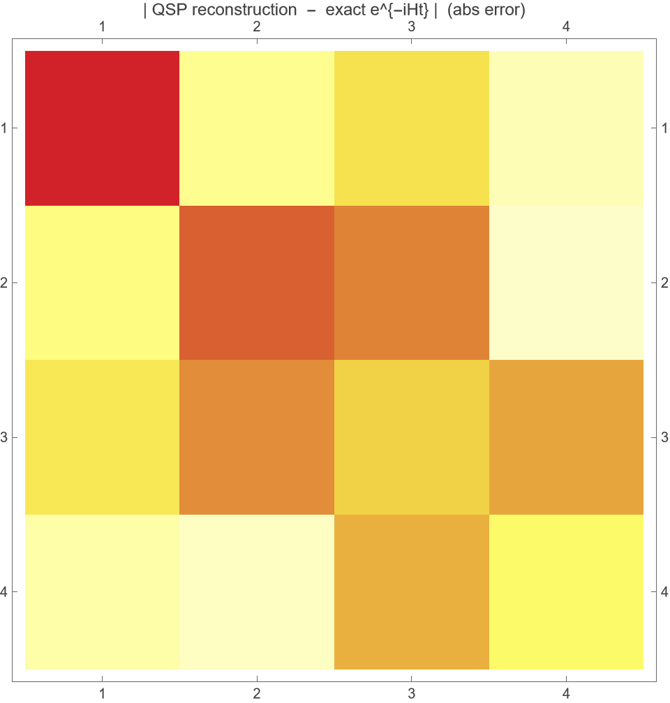
$Absolute error heatmap: QSP reconstruction vs exact e^{-iHt}$

|QSP reconstruction − exact e^−iHt| as a 4×4 error heat‑map. Largest element ≈ 10⁻⁷.

1.34×10⁻⁷max |reconstructed − exact e⁻ⁱᴴᵗ|

0.99999994normalized overlap with exact evolution

10 — THE CIRCUIT

Phases become gates

Qiskit single-qubit QSP circuit, degree 5

Qiskit — the degree‑5 QSP circuit: 6 R_Z phase gates alternating with 5 R_X signal gates on one qubit.

The QSP operators map directly onto standard rotation gates, so the abstract sequence becomes an executable circuit:

W(a) ↔ R_X(−2·arccos a) S(φ) ↔ R_Z(−2·φ)

Degree‑5 → 6 × R_Z + 5 × R_X, depth 11
Showcase: ⟨0|U|0⟩ = −0.075840 = T₅(0.6)
|abs error| vs Wolfram: 1.7×10⁻¹⁶

11 — INTEROPERABILITY

OpenQASM — the portable boundary

What it is

OpenQASM (Open Quantum Assembly) is an open, text‑based language for describing quantum circuits — an assembly language for qubits. Introduced by IBM; OpenQASM 3 adds classical control.

Why we use it

Vendor‑neutral: one circuit runs on IBM, simulators, and translates to IonQ, Quantinuum, Rigetti.
Decouples the mathematics (Wolfram) from any single SDK.
The clean hand‑off to synthesis tools like Classiq and to real hardware.

// demo1_chebyshev_d5_a0.6.qasm3 OPENQASM 3.0; include "stdgates.inc"; qubit[1] q; rz(0) q[0]; rx(-1.8545904) q[0]; rz(0) q[0]; rx(-1.8545904) q[0]; // … ×5 signal calls … rz(0) q[0];

Exported in both OpenQASM 2 & 3. rx = −2·arccos(0.6) = −1.8546.

12 — RESOURCE ESTIMATION

What will it cost to run?

Signal calls = polynomial degree = queries to the block‑encoding of H — and they dominate cost. The pipeline emits gate counts, depth and a scaling table.

degree	signal calls	R_z	R_x	depth
1	1	2	1	3
5	5	6	5	11
8	8	9	8	17
12	12	13	12	25
13	13	14	13	27

depth = 2d + 1 · IBM basis (rz, sx) compiles each block to depth 5 · opt‑3 → single U gate.

The frontier the paper sets

For Hamiltonian simulation, the optimal query complexity is:

Θ( |t| + log(1/ε) / log log(1/ε) )

This is what lets a hardware vendor answer: “given my gate budget and error rate, how large a t and how small an ε can I actually reach?”

13 — THE COMMERCIAL ECOSYSTEM

Where this creates value

The ecosystem‑layer view matters most for this paper — the same primitive is consumed differently at each layer.

🖥

Hardware vendors

Need resource estimates from QSVT to decide which problems their current and roadmap machines can reach — a benchmarking & roadmap tool.

IBMQuantinuumIonQRigettiPsiQuantumGoogle

◎

Software / middleware

Turn “give me a polynomial approximation of f” into “here is an optimized circuit.” Phase‑angle generation & synthesis is a direct product surface.

ClassiqQ‑CTRLQiskitPennyLane

☁

End‑user verticals

Consume it via cloud, without touching the math — chemistry, finance, materials and ML teams call a service.

PharmaFinanceMaterialsLogistics

Our pipeline is the QA & costing backbone each of these layers depends on: symbolic truth → machine‑precision cross‑check → portable QASM → resource scaling.

14 — CODE REFERENCE · WOLFRAM LANGUAGE

The QSP core, as written

Straight from src/QSPUnification.wl — the signal/phase operators, the QSP sequence, and the symbolic Chebyshev proof.

(* QSP signal & phase operators — Wx convention *) QSPSignalOperator[a_] := With[{th = ArcCos[a]}, {{Cos[th], I Sin[th]}, {I Sin[th], Cos[th]}}]; QSPPhaseOperator[phi_] := {{Exp[I phi], 0}, {0, Exp[-I phi]}}; (* U = S(phi0) . Prod_k W(a).S(phi_k) *) QSPUnitary[phases_List, a_] := Module[{d, w, u}, d = Length[phases] - 1; w = QSPSignalOperator[a]; u = QSPPhaseOperator[phases[[1]]]; Do[u = u . w . QSPPhaseOperator[phases[[k + 1]]], {k, 1, d}]; u]; QSPPolynomial[phases_, a_] := QSPUnitary[phases, a][[1, 1]]; (* zero phases -> P(a) = T_d(a) : proven symbolically *) ChebyshevDerivation[d_] := Module[{th, wpow, p11}, wpow = MatrixPower[QSPSignalOperator[Cos[th]], d]; p11 = FullSimplify[wpow[[1, 1]]]; FullSimplify[p11 - ChebyshevT[d, Cos[th]]] === 0];

15 — CODE REFERENCE · WOLFRAM LANGUAGE

Second quantization & phase generation

The Hamiltonian is built from the Quantum Framework's ladder operators; Jacobi–Anger sets the target; FindQSPPhases solves for the angles.

(* second quantization — Wolfram Quantum Framework *) Needs["Wolfram`QuantumFramework`"]; annFn = PacletSymbol["Wolfram/QuantumFramework", "AnnihilationOperator"]; a = annFn[size, {1}]; (* annihilation op *) aMat = Normal[a["Matrix"]]; aDag = ConjugateTranspose[aMat]; (* creation a^dag *) n = aDag . aMat; (* number n = a^dag a *) H = omega n + g (aMat + aDag); (* driven oscillator *) H = H / (Max[Abs[Eigenvalues[H]]] / 0.85); (* norm ≤ 1 *) (* Jacobi–Anger: cos(t x) via Bessel coefficients *) JacobiAngerCos[t_, K_] := BesselJ[0, t] + Sum[2 (-1)^k BesselJ[2 k, t] ChebyshevT[2 k, x], {k, 1, K}]; (* symmetric QSP phases so Re P(a) ≈ target *) cosPh = FindQSPPhases[Function[x, (1 - eta) Cos[t x]], 12, "Restarts" -> 6];

16 — CODE REFERENCE · OPENQASM

Exported OpenQASM 3 circuits

Vendor‑neutral output — every phase angle becomes an rz, every signal call an rx. Full files live in exports/qasm/.

Demo 1 — Chebyshev, degree 5

// demo1_chebyshev_d5_a0.6.qasm3 OPENQASM 3.0; include "stdgates.inc"; qubit[1] q; rz(0) q[0]; rx(-1.8545904) q[0]; // W=RX(-2·arccos a) rz(0) q[0]; rx(-1.8545904) q[0]; // … 5 signal calls total … rz(0) q[0];

Demo 2 — cos(t·a), degree 12

// demo2_cos_d12_eig0.8500.qasm3 OPENQASM 3.0; qubit[1] q; rz(-1.5707961) q[0]; // S=RZ(-2·phi) rx(-1.1096221) q[0]; rz(-1.31e-06) q[0]; rx(-1.1096221) q[0]; rz(7.85e-05) q[0]; rx(-1.1096221) q[0]; // … 12 calls, symmetric … rz(-1.5707961) q[0];

17 — SUMMARY

Paper → verified circuits, end to end

35/35proof‑audit checks

6.1×10⁻¹⁶Wolfram ↔ Qiskit

0.99999994e⁻ⁱᴴᵗ overlap

Deliverables

Symbolic derivation & numerical verification
Gate circuits + OpenQASM 2 & 3
Circuit & Wolfram visualizations
Resource estimation + scaling table
Interactive notebook QSPUnification.nb

Built with

·

· OpenQASM

Wolfram Mathematica 14.3

Wolfram Quantum Framework

Amp — Mathematica skill

Qiskit + Aer

Repository

github.com/zuwasi/qsp‑qsvt‑unification‑pipeline

Quantum Signal Processing · Chebyshev · Hamiltonian Simulation · OpenQASM

18 — THANK YOU

Thank you
for watching

The complete project — code & documentation — is available to the public under the MIT License in this repository:

github.com/zuwasi/qsp-qsvt-unification-pipeline →

Feel free to use, modify, improve, give feedback, and submit Pull Requests.

Author

Daniel Liezrowice

LinkedIn →

Grand Unification ofQuantum Algorithms

ESL — Engineering Software Lab

Daniel Liezrowice

One primitive, most known quantum algorithms

The core insight

Why it matters commercially

The workflow we built

Optimal Mathematica, driven by Amp

Wolfram Quantum Framework

Headless .wl / .wls scripts

Quantum Signal Processing in one screen

Signal & phase operators (Wx convention)

The QSP sequence & its response

QSP ⇒ Chebyshev polynomials

Every identity, checked numerically

From cos & sin to e−iHt

Eigenvalue transform & reconstruction

Phases become gates

OpenQASM — the portable boundary

What it is

Why we use it

What will it cost to run?

The frontier the paper sets

Where this creates value

Hardware vendors

Software / middleware

End‑user verticals

The QSP core, as written

Second quantization & phase generation

Exported OpenQASM 3 circuits

Paper → verified circuits, end to end

Deliverables

Built with

Thank youfor watching

Daniel Liezrowice

Grand Unification of
Quantum Algorithms

From cos & sin to e^−iHt

Thank you
for watching